77. The Aiyagari Model with Endogenous Grid Method#
In addition to what’s included in base Anaconda, we need to install JAX
!pip install quantecon jax
77.1. Overview#
This lecture combines two important computational methods in macroeconomics:
The Aiyagari model [Aiyagari, 1994] - a heterogeneous agent model with incomplete markets
The endogenous grid method (EGM) [Carroll, 2006] - an efficient algorithm for solving dynamic programming problems
In the standard Aiyagari lecture, we solved the household problem using Howard policy iteration (a value function iteration variant) and computed aggregate capital using the stationary distribution of the finite Markov chain.
In this lecture, we take a different approach:
We use the endogenous grid method to solve the household problem via the Euler equation, avoiding costly root-finding operations
We compute aggregate capital by simulation rather than calculating the stationary distribution analytically
These modifications make the solution method faster and more flexible, especially when dealing with more complex models.
77.1.1. References#
The primary references for this lecture are:
[Aiyagari, 1994] for the economic model
[Carroll, 2006] for the endogenous grid method
Chapter 18 of [Ljungqvist and Sargent, 2018] for textbook treatment
77.1.2. Preliminaries#
We use the following imports:
import quantecon as qe
import matplotlib.pyplot as plt
import jax
import jax.numpy as jnp
from typing import NamedTuple
from scipy.optimize import bisect
import numpy as np
from numba import jit
Matplotlib is building the font cache; this may take a moment.
We will use 64-bit floats with JAX in order to increase precision.
jax.config.update("jax_enable_x64", True)
77.2. The Economy#
77.2.1. Households#
Infinitely lived households face idiosyncratic income shocks and a borrowing constraint.
The savings problem faced by a typical household is
subject to
where
\(c_t\) is current consumption
\(a_t\) is assets
\(z_t\) is an exogenous component of labor income (stochastic employment status)
\(w\) is a wage rate
\(r\) is a net interest rate
\(B\) is the maximum amount that the agent is allowed to borrow
The exogenous process \(\{z_t\}\) follows a finite state Markov chain with stochastic matrix \(\Pi\).
The Euler equation for this problem is
or, in terms of assets,
where \(a'(a, z)\) is the optimal savings policy function.
77.2.2. Firms#
Firms produce output by hiring capital and labor under constant returns to scale.
The representative firm’s output is
where
\(A\) and \(\alpha\) are parameters with \(A > 0\) and \(\alpha \in (0, 1)\)
\(K\) is aggregate capital
\(N\) is total labor supply (normalized to 1)
These parameters are stored in the following namedtuple:
class Firm(NamedTuple):
    A: float = 1.0    # Total factor productivity
    N: float = 1.0    # Total labor supply
    α: float = 0.33   # Capital share
    δ: float = 0.05   # Depreciation rate
From the firm’s first-order condition, the inverse demand for capital is
def r_given_k(K, firm):
    """
    Inverse demand curve for capital.
    """
    A, N, α, δ = firm
    return A * α * (N / K)**(1 - α) - δ
The equilibrium wage rate as a function of \(r\) is
def r_to_w(r, firm):
    """
    Equilibrium wages associated with a given interest rate r.
    """
    A, N, α, δ = firm
    return A * (1 - α) * (A * α / (r + δ))**(α / (1 - α))
77.2.3. Equilibrium#
A stationary rational expectations equilibrium (SREE) consists of prices and policies such that:
Households optimize given prices
Firms maximize profits given prices
Markets clear: aggregate capital supply equals aggregate capital demand
Aggregate quantities are constant over time
77.3. Implementation with EGM#
77.3.1. Household primitives#
First we set up the household parameters and grids:
class Household(NamedTuple):
    β: float            # Discount factor
    a_grid: jnp.ndarray # Asset grid
    z_grid: jnp.ndarray # Exogenous states
    Π: jnp.ndarray      # Transition matrix

def create_household(β=0.96,                      # Discount factor
                     Π=[[0.9, 0.1], [0.1, 0.9]],  # Markov chain
                     z_grid=[0.1, 1.0],           # Exogenous states
                     a_min=1e-10, a_max=50,       # Asset grid
                     a_size=200):
    """
    Create a Household namedtuple with custom grids.
    """
    a_grid = jnp.linspace(a_min, a_max, a_size)
    z_grid, Π = map(jnp.array, (z_grid, Π))
    return Household(β=β, a_grid=a_grid, z_grid=z_grid, Π=Π)
For utility, we assume \(u(c) = \log(c)\), which gives us \(u'(c) = 1/c\) and \((u')^{-1}(x) = 1/x\).
@jax.jit
def u(c):
    return jnp.log(c)

@jax.jit
def u_prime(c):
    return 1 / c

@jax.jit
def u_prime_inv(x):
    return 1 / x
Here’s a namedtuple for prices:
class Prices(NamedTuple):
    r: float = 0.01  # Interest rate
    w: float = 1.0   # Wages
77.3.2. The EGM operator#
The key insight of EGM is to avoid root-finding by choosing the asset grid exogenously and computing the consumption values directly from the Euler equation.
The Coleman-Reffett operator using EGM works as follows:
Start with a consumption policy function \(\sigma\) represented on an exogenous grid of assets \(\{a_i\}\)
For each asset level \(a_i\) and employment state \(z_j\):
Compute the right-hand side of the Euler equation: $\(\text{RHS} = \beta (1 + r) \sum_{z'} \Pi(z_j, z') u'(\sigma(a_i, z'))\)$
Use the inverse marginal utility to get current consumption: $\(c_{ij} = (u')^{-1}(\text{RHS})\)$
Compute the endogenous income level: $\(y_{ij} = c_{ij} + a_i\)$
Reconstruct the new policy \(K\sigma\) on the original asset grid using interpolation
@jax.jit
def K_egm(σ, household, prices):
    """
    The Coleman-Reffett operator using EGM for the Aiyagari model.

    Parameters
    ----------
    σ : array_like(float, ndim=2)
        Current consumption policy, where σ[i, j] is consumption
        when assets are a_grid[i] and employment state is z_grid[j]
    household : Household
        Household parameters and grids
    prices : Prices
        Interest rate and wage

    Returns
    -------
    σ_new : array_like(float, ndim=2)
        Updated consumption policy on the same grid
    """
    # Unpack
    β, a_grid, z_grid, Π = household
    a_size, z_size = len(a_grid), len(z_grid)
    r, w = prices

    # Allocate memory for new consumption
    σ_new = jnp.zeros((a_size, z_size))

    # For each current employment state
    for j in range(z_size):
        # Step 1: Use a_grid as exogenous grid for tomorrow's assets (a')
        # Compute expectation: E[u'(c(a', z')) | z=z_j]
        Eu_prime = jnp.zeros(a_size)
        for jp in range(z_size):
            Eu_prime += Π[j, jp] * u_prime(σ[:, jp])

        # Step 2: Get consumption on endogenous grid using Euler equation
        c_endo = u_prime_inv(β * (1 + r) * Eu_prime)

        # Step 3: Compute endogenous asset grid for today
        # From budget constraint: a' = (1+r)a + wz - c
        # Solving for a: a = (c + a' - wz) / (1+r)
        a_endo = (c_endo + a_grid - w * z_grid[j]) / (1 + r)

        # Step 4: Interpolate back to exogenous asset grid
        # Handle borrowing constraint
        for i, a in enumerate(a_grid):
            if a < a_endo[0]:
                # Below minimum of endogenous grid - consume all income
                σ_new = σ_new.at[i, j].set(w * z_grid[j] + (1 + r) * a - a_grid[0])
            else:
                # Interpolate
                σ_new = σ_new.at[i, j].set(jnp.interp(a, a_endo, c_endo))

    return σ_new
Let’s also create a more efficient JIT-compiled version:
@jax.jit
def K_egm_jit(σ, household, prices):
    """
    Vectorized JIT-compiled version of the EGM operator.
    """
    # Unpack
    β, a_grid, z_grid, Π = household
    a_size, z_size = len(a_grid), len(z_grid)
    r, w = prices

    # Compute expectation: E[u'(c(a', z')) | z]
    # Eu_prime[i, j] = sum_jp Π[j, jp] * u'(σ[i, jp])
    Eu_prime = (Π @ u_prime(σ).T).T  # (a_size, z_size)

    # Apply Euler equation to get consumption on endogenous grid
    c_endo = u_prime_inv(β * (1 + r) * Eu_prime)  # (a_size, z_size)

    # Compute endogenous asset grid: a = (c + a' - wz) / (1+r)
    # a_endo[i, j] is today's assets when tomorrow's assets are a_grid[i]
    # and today's employment is z_grid[j]
    a_endo = (c_endo + a_grid[:, None] - w * z_grid[None, :]) / (1 + r)

    # Interpolate back to exogenous grid
    # For each employment state j, interpolate from (a_endo[:, j], c_endo[:, j])
    # to get consumption at exogenous grid points a_grid

    def interpolate_policy(j):
        # Handle borrowing constraint
        # If a < min(a_endo), consume everything except minimum savings
        return jnp.where(
            a_grid < a_endo[0, j],
            w * z_grid[j] + (1 + r) * a_grid - a_grid[0],
            jnp.interp(a_grid, a_endo[:, j], c_endo[:, j])
        )

    σ_new = jax.vmap(interpolate_policy)(jnp.arange(z_size))

    return σ_new.T  # (a_size, z_size)
77.3.3. Solving the household problem#
We solve for the optimal policy by iterating the EGM operator to convergence:
def solve_household_egm(household, prices,
                        tol=1e-5, max_iter=1000, verbose=False):
    """
    Solve the household problem using EGM iteration.

    Returns the optimal consumption policy σ[i,j] where i indexes
    assets and j indexes employment states.
    """
    β, a_grid, z_grid, Π = household
    a_size, z_size = len(a_grid), len(z_grid)

    # Initial guess: consume a fraction of income
    r, w = prices
    a_mesh = a_grid[:, None]
    z_mesh = z_grid[None, :]
    income = w * z_mesh + (1 + r) * a_mesh
    σ = 0.5 * income

    # Iterate until convergence
    for i in range(max_iter):
        σ_new = K_egm_jit(σ, household, prices)
        error = jnp.max(jnp.abs(σ_new - σ))
        σ = σ_new

        if verbose and i % 50 == 0:
            print(f"Iteration {i}, error = {error:.6f}")

        if error < tol:
            if verbose:
                print(f"Converged in {i} iterations")
            break

    return σ
Let’s test this on an example:
# Create household and prices
household = create_household()
prices = Prices(r=0.01, w=1.0)

print(f"Solving household problem with r={prices.r}, w={prices.w}")

# Solve
with qe.Timer():
    σ_star = solve_household_egm(household, prices, verbose=True)
Solving household problem with r=0.01, w=1.0
Iteration 0, error = 7.907526
Iteration 50, error = 0.006472
Iteration 100, error = 0.000021
Converged in 106 iterations
0.83 seconds elapsed
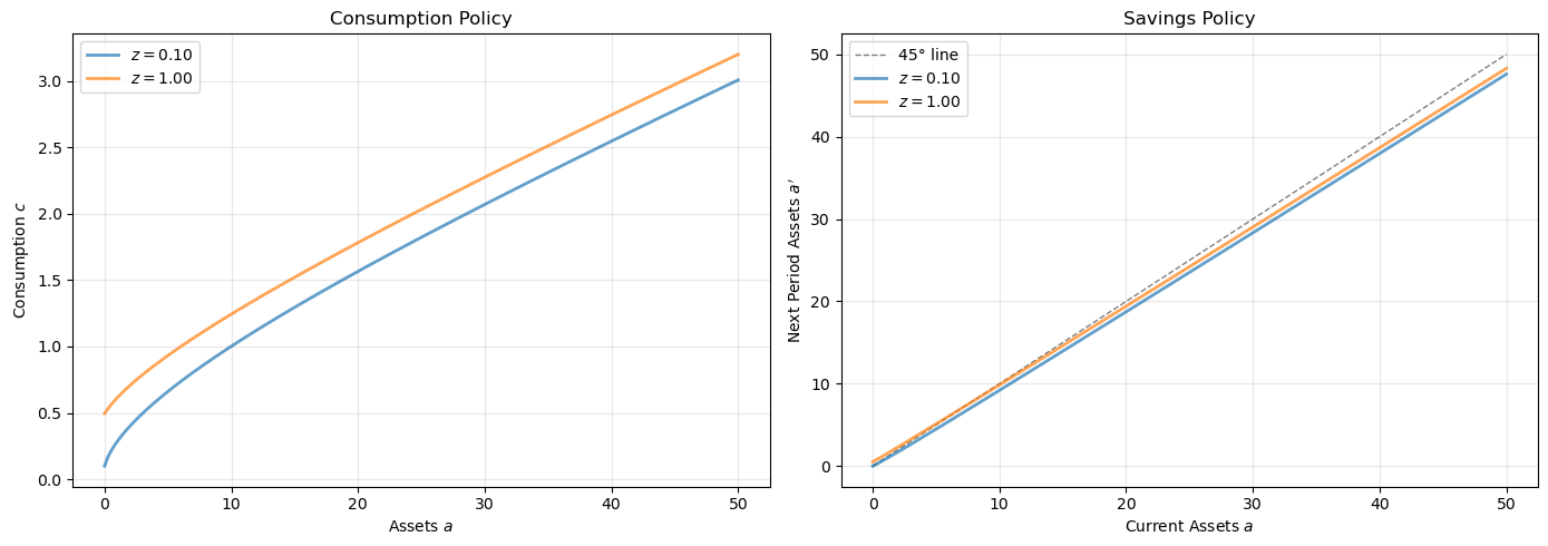
Let’s plot the resulting policy functions:
β, a_grid, z_grid, Π = household
r, w = prices

# Convert consumption policy to savings policy
a_mesh = a_grid[:, None]
z_mesh = z_grid[None, :]
income = w * z_mesh + (1 + r) * a_mesh
savings = income - σ_star

fig, axes = plt.subplots(1, 2, figsize=(14, 5))

# Plot consumption policy
ax = axes[0]
for j, z in enumerate(z_grid):
    ax.plot(a_grid, σ_star[:, j], label=f'$z={z:.2f}$', lw=2, alpha=0.7)
ax.set_xlabel('Assets $a$')
ax.set_ylabel('Consumption $c$')
ax.set_title('Consumption Policy')
ax.legend()
ax.grid(alpha=0.3)

# Plot savings policy
ax = axes[1]
ax.plot(a_grid, a_grid, 'k--', lw=1, alpha=0.5, label='45° line')
for j, z in enumerate(z_grid):
    ax.plot(a_grid, savings[:, j], label=f'$z={z:.2f}$', lw=2, alpha=0.7)
ax.set_xlabel('Current Assets $a$')
ax.set_ylabel('Next Period Assets $a\'$')
ax.set_title('Savings Policy')
ax.legend()
ax.grid(alpha=0.3)

plt.tight_layout()
plt.show()
77.4. Computing Aggregate Capital by Simulation#
Instead of computing the stationary distribution of the Markov chain analytically, we compute aggregate capital by simulating a large number of households.
This approach:
Is more flexible (works with continuous shocks, non-linear policies, etc.)
Avoids storing and manipulating large transition matrices
Is conceptually simpler
@jax.jit
def simulate_households(σ, household, prices,
                       num_households=10_000,
                       num_periods=1000,
                       seed=42):
    """
    Simulate a cross-section of households and compute average assets.

    Parameters
    ----------
    σ : array_like(float)
        Consumption policy function
    household : Household
        Household parameters
    prices : Prices
        Interest rate and wage
    num_households : int
        Number of households to simulate
    num_periods : int
        Number of periods to simulate (we use the last period)
    seed : int
        Random seed

    Returns
    -------
    mean_assets : float
        Average asset holdings across households
    """
    β, a_grid, z_grid, Π = household
    r, w = prices
    z_size = len(z_grid)

    # Initialize random states
    key = jax.random.PRNGKey(seed)

    # Initial asset distribution (start everyone at the middle of the grid)
    a_init_idx = len(a_grid) // 2
    assets = jnp.ones(num_households) * a_grid[a_init_idx]

    # Initial employment state distribution (draw from stationary dist)
    # For simplicity, start everyone in state 0
    z_indices = jnp.zeros(num_households, dtype=int)

    # Simulate forward
    for t in range(num_periods):
        # Generate random shocks for employment transitions
        key, subkey = jax.random.split(key)
        unif = jax.random.uniform(subkey, shape=(num_households,))

        # Update employment states based on transition matrix
        z_indices_new = jnp.zeros(num_households, dtype=int)
        for i in range(num_households):
            z_idx = z_indices[i]
            # Cumulative probabilities
            cum_probs = jnp.cumsum(Π[z_idx, :])
            # Find which state to transition to
            z_indices_new = z_indices_new.at[i].set(
                jnp.searchsorted(cum_probs, unif[i])
            )
        z_indices = z_indices_new

        # Get current income
        z_current = z_grid[z_indices]
        income = w * z_current + (1 + r) * assets

        # Interpolate consumption policy
        consumption = jnp.zeros(num_households)
        for i in range(num_households):
            # Use 2D interpolation: interp over assets for each z
            consumption = consumption.at[i].set(
                jnp.interp(assets[i], a_grid, σ[:, z_indices[i]])
            )

        # Update assets
        assets = income - consumption
        assets = jnp.maximum(assets, a_grid[0])  # Enforce borrowing constraint

    return jnp.mean(assets)
The function above is fully JIT-compiled but might be slow for the loops. Let’s create a more efficient version using jax.lax.fori_loop:
def simulate_assets_efficient(σ, household, prices,
                              num_households=50_000,
                              num_periods=1000,
                              burn_in=500,
                              seed=42):
    """
    Efficient simulation using numpy (numba would be even better but
    we'll keep it simple with numpy for now).
    """
    β, a_grid, z_grid, Π = household
    r, w = prices
    z_size = len(z_grid)

    # Convert to numpy for simulation
    a_grid_np = np.array(a_grid)
    z_grid_np = np.array(z_grid)
    Π_np = np.array(Π)
    σ_np = np.array(σ)

    # Set random seed
    np.random.seed(seed)

    # Initialize
    a_init_idx = len(a_grid_np) // 2
    assets = np.ones(num_households) * a_grid_np[a_init_idx]
    z_indices = np.zeros(num_households, dtype=int)

    # Simulate
    for t in range(num_periods):
        # Draw employment shocks
        unif = np.random.uniform(size=num_households)

        # Update employment states
        for i in range(num_households):
            cum_probs = np.cumsum(Π_np[z_indices[i], :])
            z_indices[i] = np.searchsorted(cum_probs, unif[i])

        # Compute income
        z_current = z_grid_np[z_indices]
        income = w * z_current + (1 + r) * assets

        # Interpolate consumption policy
        # Note: np.interp extrapolates using boundary values, which can cause
        # issues if assets go far outside the grid. The grid should be large
        # enough to cover the range of assets in equilibrium.
        consumption = np.array([
            np.interp(assets[i], a_grid_np, σ_np[:, z_indices[i]])
            for i in range(num_households)
        ])

        # Update assets
        assets = income - consumption
        assets = np.maximum(assets, a_grid_np[0])  # Enforce borrowing constraint

        # Clip assets to grid maximum to prevent extrapolation issues
        # In equilibrium, assets should stay within the grid if a_max is large enough
        assets = np.minimum(assets, a_grid_np[-1])

    return np.mean(assets)
Now we can compute capital supply for given prices:
def capital_supply(household, prices,
                  num_households=50_000,
                  num_periods=1000):
    """
    Compute aggregate capital supply by simulation.
    """
    # Solve household problem
    σ = solve_household_egm(household, prices)

    # Simulate to get mean assets
    mean_assets = simulate_assets_efficient(
        σ, household, prices,
        num_households=num_households,
        num_periods=num_periods
    )

    return mean_assets
Let’s test it:
household = create_household()
prices = Prices(r=0.01, w=1.0)

print("Computing capital supply via simulation...")
with qe.Timer():
    K_supply = capital_supply(household, prices,
                             num_households=10_000,
                             num_periods=500)

print(f"Capital supply: {K_supply:.4f}")
Computing capital supply via simulation...
39.74 seconds elapsed
Capital supply: 2.6035
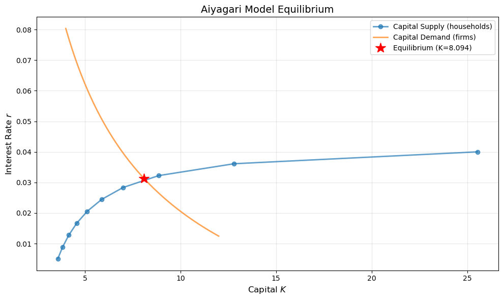
77.5. Computing Equilibrium#
Now we can compute the equilibrium by finding the interest rate where capital supply equals capital demand.
The equilibrium mapping is:
where \(G(K)\) computes:
Prices \((r, w)\) from firm FOCs given \(K\)
Household optimal policy given prices
Aggregate capital via simulation
def G(K, firm, household,
      num_households=10_000,
      num_periods=500):
    """
    The equilibrium mapping K -> K'.
    """
    # Get prices from firm problem
    r = r_given_k(K, firm)
    w = r_to_w(r, firm)
    prices = Prices(r=r, w=w)

    # Compute capital supply
    K_supply = capital_supply(household, prices,
                             num_households=num_households,
                             num_periods=num_periods)

    return K_supply
We can compute equilibrium using bisection:
def compute_equilibrium(firm, household,
                       K_min=1.0, K_max=20.0,
                       num_households=10_000,
                       num_periods=500,
                       xtol=1e-3):
    """
    Compute equilibrium capital stock using bisection.
    """
    def excess_demand(K):
        K_supply = G(K, firm, household,
                    num_households=num_households,
                    num_periods=num_periods)
        return K - K_supply

    K_star = bisect(excess_demand, K_min, K_max, xtol=xtol)
    return K_star
Let’s compute the equilibrium:
firm = Firm()
household = create_household()

print("Computing equilibrium capital stock...")
print("(This may take a few minutes due to simulation)")

with qe.Timer():
    K_star = compute_equilibrium(
        firm, household,
        K_min=4.0, K_max=12.0,
        num_households=5_000,
        num_periods=400,
        xtol=5e-2
    )

print(f"\nEquilibrium capital: {K_star:.4f}")

# Get equilibrium prices
r_star = r_given_k(K_star, firm)
w_star = r_to_w(r_star, firm)
print(f"Equilibrium interest rate: {r_star:.4f}")
print(f"Equilibrium wage: {w_star:.4f}")
Computing equilibrium capital stock...
(This may take a few minutes due to simulation)
159.55 seconds elapsed

Equilibrium capital: 8.0938
Equilibrium interest rate: 0.0313
Equilibrium wage: 1.3359
77.5.1. Visualizing equilibrium#
Let’s plot the supply and demand curves:
# Compute supply curve (capital as function of r)
r_vals = np.linspace(0.005, 0.04, 10)
K_supply_vals = []

print("Computing supply curve...")
for r in r_vals:
    w = r_to_w(r, firm)
    prices = Prices(r=r, w=w)
    K_s = capital_supply(household, prices,
                        num_households=5_000,
                        num_periods=300)
    K_supply_vals.append(K_s)
    print(f"  r={r:.4f}: K={K_s:.3f}")

# Demand curve
K_vals = np.linspace(4, 12, 50)
r_demand_vals = r_given_k(K_vals, firm)

# Plot
fig, ax = plt.subplots(figsize=(10, 6))

ax.plot(K_supply_vals, r_vals, 'o-', lw=2,
        alpha=0.7, label='Capital Supply (households)',
        markersize=6)
ax.plot(K_vals, r_demand_vals, lw=2,
        alpha=0.7, label='Capital Demand (firms)')

# Mark equilibrium
ax.plot(K_star, r_star, 'r*', markersize=15,
        label=f'Equilibrium (K={K_star:.3f})', zorder=5)

ax.set_xlabel('Capital $K$', fontsize=12)
ax.set_ylabel('Interest Rate $r$', fontsize=12)
ax.set_title('Aiyagari Model Equilibrium', fontsize=14)
ax.legend(fontsize=10)
ax.grid(alpha=0.3)

plt.tight_layout()
plt.show()
Computing supply curve...
r=0.0050: K=3.580
r=0.0089: K=3.836
r=0.0128: K=4.160
r=0.0167: K=4.574
r=0.0206: K=5.121
r=0.0244: K=5.878
r=0.0283: K=6.996
r=0.0322: K=8.855
r=0.0361: K=12.804
r=0.0400: K=25.534
77.6. Wealth Distribution#
One advantage of the simulation approach is that we can easily examine the wealth distribution:
def simulate_wealth_distribution(household, prices,
                                num_households=50_000,
                                num_periods=1000):
    """
    Simulate and return the cross-sectional wealth distribution.
    """
    # Solve household problem
    σ = solve_household_egm(household, prices)

    β, a_grid, z_grid, Π = household
    r, w = prices

    # Convert to numpy
    a_grid_np = np.array(a_grid)
    z_grid_np = np.array(z_grid)
    Π_np = np.array(Π)
    σ_np = np.array(σ)

    np.random.seed(42)

    # Initialize
    a_init_idx = len(a_grid_np) // 2
    assets = np.ones(num_households) * a_grid_np[a_init_idx]
    z_indices = np.zeros(num_households, dtype=int)

    # Simulate
    for t in range(num_periods):
        unif = np.random.uniform(size=num_households)

        for i in range(num_households):
            cum_probs = np.cumsum(Π_np[z_indices[i], :])
            z_indices[i] = np.searchsorted(cum_probs, unif[i])

        z_current = z_grid_np[z_indices]
        income = w * z_current + (1 + r) * assets

        consumption = np.array([
            np.interp(assets[i], a_grid_np, σ_np[:, z_indices[i]])
            for i in range(num_households)
        ])

        assets = income - consumption
        assets = np.maximum(assets, a_grid_np[0])

    return assets, z_indices

# Simulate wealth distribution at equilibrium
prices_star = Prices(r=r_star, w=w_star)
assets_dist, z_dist = simulate_wealth_distribution(
    household, prices_star,
    num_households=10_000,
    num_periods=800
)

# Plot
fig, axes = plt.subplots(1, 2, figsize=(14, 5))

# Histogram
ax = axes[0]
ax.hist(assets_dist, bins=50, density=True, alpha=0.7, edgecolor='black')
ax.axvline(np.mean(assets_dist), color='red', linestyle='--',
          linewidth=2, label=f'Mean = {np.mean(assets_dist):.3f}')
ax.axvline(np.median(assets_dist), color='orange', linestyle='--',
          linewidth=2, label=f'Median = {np.median(assets_dist):.3f}')
ax.set_xlabel('Assets', fontsize=12)
ax.set_ylabel('Density', fontsize=12)
ax.set_title('Wealth Distribution', fontsize=14)
ax.legend()
ax.grid(alpha=0.3)

# Lorenz curve
ax = axes[1]
sorted_assets = np.sort(assets_dist)
cum_wealth = np.cumsum(sorted_assets) / np.sum(sorted_assets)
cum_pop = np.linspace(0, 1, len(sorted_assets))

ax.plot(cum_pop, cum_wealth, lw=2, label='Lorenz Curve')
ax.plot([0, 1], [0, 1], 'k--', lw=1, alpha=0.5, label='Perfect Equality')
ax.set_xlabel('Cumulative Population Share', fontsize=12)
ax.set_ylabel('Cumulative Wealth Share', fontsize=12)
ax.set_title('Lorenz Curve', fontsize=14)
ax.legend()
ax.grid(alpha=0.3)

plt.tight_layout()
plt.show()

# Compute Gini coefficient
gini = 1 - 2 * np.trapz(cum_wealth, cum_pop)
print(f"\nGini coefficient: {gini:.4f}")
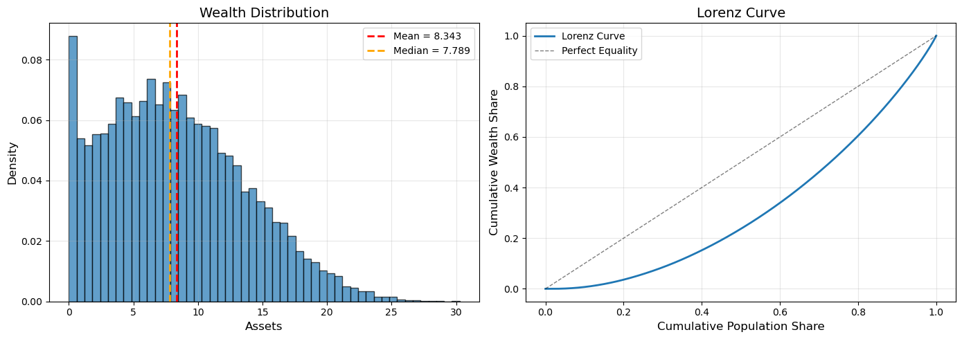
Gini coefficient: 0.3649
/tmp/ipykernel_2839/1845471123.py:89: DeprecationWarning: `trapz` is deprecated. Use `trapezoid` instead, or one of the numerical integration functions in `scipy.integrate`.
  gini = 1 - 2 * np.trapz(cum_wealth, cum_pop)
77.7. Summary and Comparison#
This lecture demonstrated how to solve the Aiyagari model using:
Endogenous Grid Method (EGM) for the household problem
Avoids costly root-finding by working backwards from the Euler equation
Directly computes consumption from marginal utility
More efficient than value function iteration
Simulation for computing aggregate capital
Simulates a large cross-section of households
More flexible than analytical stationary distributions
Allows easy computation of wealth inequality measures
77.7.1. Comparison with standard approach#
Compared to the standard Aiyagari lecture:
Advantages:
EGM is faster than Howard iteration (no root-finding needed)
Simulation is more flexible (works with continuous shocks, non-linear policies)
Easy to compute distributional statistics (Gini, percentiles, etc.)
Simpler to extend to more complex models
Disadvantages:
Simulation requires large number of households for accuracy
Equilibrium computation is slower due to simulation
Less precise than analytical stationary distribution
77.7.2. Extensions#
This framework can be easily extended to:
Continuous income shocks (e.g., lognormal)
More complex preference specifications
Aggregate shocks and heterogeneous agent New Keynesian (HANK) models
Life-cycle models with age-dependent policies
77.8. Exercises#
Exercise 77.1
Compare the speed and accuracy of EGM vs. Howard iteration for solving the household problem.
Implement a version that uses Howard iteration (you can adapt code from the standard Aiyagari lecture)
Time both methods and compare the resulting policies
Which method is faster? Are the policies identical?
Exercise 77.2
Study how the wealth distribution changes with the discount factor \(\beta\).
Compute equilibria for \(\beta \in \{0.94, 0.95, 0.96, 0.97\}\)
For each \(\beta\), compute and plot the wealth distribution
How does the Gini coefficient change with \(\beta\)?
Explain the economic intuition
Exercise 77.3
The simulation method introduced in this lecture uses a fixed number of periods. Investigate the impact of this choice:
Vary
num_periodsfrom 200 to 2000For each value, compute the mean assets multiple times with different random seeds
Plot the standard deviation of the capital estimate as a function of
num_periodsWhat is the trade-off between accuracy and computational cost?
Exercise 77.4
Extend the model to include a third employment state (e.g., unemployed, part-time, full-time):
Set up a 3-state Markov chain with appropriate transition probabilities
Define income levels for each state
Re-compute the equilibrium
How does the additional heterogeneity affect the wealth distribution?