71. Lake Model with an Endogenous Job Finding Rate#
In addition to what’s in Anaconda, this lecture will need the following libraries:
!pip install quantecon jax
71.1. Overview#
This lecture is a continuation of the lake model lecture.
We recommend you read that lecture first before proceeding with this one.
In the previous lecture, we studied a lake model of unemployment and employment where the transition rates between states were exogenous parameters.
In this lecture, we extend the model by making the job finding rate endogenous.
Specifically, the transition rate from unemployment to employment will be determined by the McCall search model [McCall, 1970].
Let’s start with some imports:
import matplotlib.pyplot as plt
import jax
import jax.numpy as jnp
from typing import NamedTuple
from quantecon.distributions import BetaBinomial
from functools import partial
import jax.scipy.stats as stats
71.2. Set Up#
The basic structure of the model will be as discussed in the lake model lecture.
The only difference is that the hiring rate is endogenous, determined by the decisions of optimizing agents inhabiting a McCall search model [McCall, 1970] with IID wage offers and job separation at rate \(\alpha\).
71.2.1. Reservation wage#
In the model, the optimal policy is characterized by a reservation wage \(\bar w\)
If the wage offer \(w\) in hand is greater than or equal to \(\bar w\), then the worker accepts.
Otherwise, the worker rejects.
The reservation wage depends on the wage offer distribution and the parameters
\(\alpha\), the separation rate
\(\beta\), the discount factor
\(\gamma\), the offer arrival rate
\(c\), unemployment compensation
The wage offer distribution will be a discretized version of a lognormal distribution.
We first define a function to create such a discrete distribution.
def create_wage_distribution(
        max_wage: float,
        wage_grid_size: int,
        log_wage_mean: float
    ):
    """
    Creates a discretized version of a lognormal density LN(log(m),1), where
    m is log_wage_mean.

    """
    w_vec_temp = jnp.linspace(1e-8, max_wage, wage_grid_size + 1)
    cdf = stats.norm.cdf(
        jnp.log(w_vec_temp), loc=jnp.log(log_wage_mean), scale=1
    )
    pdf = cdf[1:] - cdf[:-1]
    p_vec = pdf / pdf.sum()
    w_vec = (w_vec_temp[1:] + w_vec_temp[:-1]) / 2
    return w_vec, p_vec
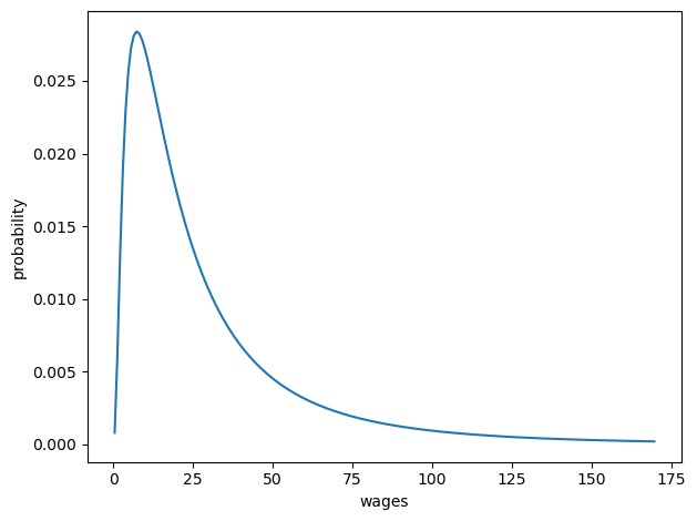
The cell below creates a discretized \(LN(\log(20),1)\) wage distribution and plots it.
w_vec, p_vec = create_wage_distribution(170, 200, 20)

fig, ax = plt.subplots()
ax.plot(w_vec, p_vec)
ax.set_xlabel('wages')
ax.set_ylabel('probability')
plt.tight_layout()
plt.show()
Now we organize the code for solving the McCall model, given a set of parameters.
For background on the model and our solution method, see the lecture on the McCall model with separation
Our first step is to define the utility function and the McCall model data structure.
def u(c, σ=2.0):
    return jnp.where(c > 0, (c**(1 - σ) - 1) / (1 - σ), -10e6)


class McCallModel(NamedTuple):
    """
    Stores the parameters for the McCall search model
    """
    α: float            # Job separation rate
    β: float            # Discount rate
    γ: float            # Job offer rate
    c: float            # Unemployment compensation
    σ: float            # Utility parameter
    w_vec: jnp.ndarray  # Possible wage values
    p_vec: jnp.ndarray  # Probabilities over w_vec


def create_mccall_model(
        α=0.2, β=0.98, γ=0.7, c=6.0, σ=2.0,
        w_vec=None,
        p_vec=None
    ) -> McCallModel:
    if w_vec is None:
        n = 60  # Number of possible outcomes for wage
        # Wages between 10 and 20
        w_vec = jnp.linspace(10, 20, n)
        a, b = 600, 400  # Shape parameters
        dist = BetaBinomial(n-1, a, b)
        p_vec = jnp.array(dist.pdf())
    return McCallModel(
        α=α, β=β, γ=γ, c=c, σ=σ, w_vec=w_vec, p_vec=p_vec
    )
Next, we implement the Bellman operator
def T(mcm: McCallModel, V, U):
    """
    Update the Bellman equations.
    """
    α, β, γ, c, σ = mcm.α, mcm.β, mcm.γ, mcm.c, mcm.σ
    w_vec, p_vec = mcm.w_vec, mcm.p_vec

    V_new = u(w_vec, σ) + β * ((1 - α) * V + α * U)
    U_new = u(c, σ) + β * (1 - γ) * U + β * γ * (jnp.maximum(U, V) @ p_vec)

    return V_new, U_new
Now we define the value function iteration solver.
We’ll use a compiled while loop for extra speed.
@jax.jit
def solve_mccall_model(mcm: McCallModel, tol=1e-5, max_iter=2000):
    """
    Iterates to convergence on the Bellman equations.
    """
    def cond(state):
        V, U, i, error = state
        return jnp.logical_and(error > tol, i < max_iter)

    def update(state):
        V, U, i, error = state
        V_new, U_new = T(mcm, V, U)
        error_1 = jnp.max(jnp.abs(V_new - V))
        error_2 = jnp.abs(U_new - U)
        error_new = jnp.maximum(error_1, error_2)
        return V_new, U_new, i + 1, error_new

    # Initial state
    V_init = jnp.ones(len(mcm.w_vec))
    U_init = 1.0
    i_init = 0
    error_init = tol + 1

    init_state = (V_init, U_init, i_init, error_init)
    V_final, U_final, _, _ = jax.lax.while_loop(
        cond, update, init_state
    )
    return V_final, U_final
71.2.2. Lake model code#
We also need the lake model functions from the previous lecture to compute steady state unemployment rates:
class LakeModel(NamedTuple):
    """
    Parameters for the lake model
    """
    λ: float
    α: float
    b: float
    d: float
    A: jnp.ndarray
    R: jnp.ndarray
    g: float


def create_lake_model(
        λ: float = 0.283,     # job finding rate
        α: float = 0.013,     # separation rate
        b: float = 0.0124,    # birth rate
        d: float = 0.00822    # death rate
    ) -> LakeModel:
    """
    Create a LakeModel instance with default parameters.

    Computes and stores the transition matrices A and R,
    and the labor force growth rate g.

    """
    # Compute growth rate
    g = b - d

    # Compute transition matrix A
    A = jnp.array([
        [(1-d) * (1-λ) + b, (1-d) * α + b],
        [(1-d) * λ,         (1-d) * (1-α)]
    ])

    # Compute normalized transition matrix R
    R = A / (1 + g)

    return LakeModel(λ=λ, α=α, b=b, d=d, A=A, R=R, g=g)


@jax.jit
def rate_steady_state(model: LakeModel) -> jnp.ndarray:
    r"""
    Finds the steady state of the system :math:`x_{t+1} = R x_{t}`
    by computing the eigenvector corresponding to the largest eigenvalue.

    By the Perron-Frobenius theorem, since :math:`R` is a non-negative
    matrix with columns summing to 1 (a stochastic matrix), the largest
    eigenvalue equals 1 and the corresponding eigenvector gives the steady state.
    """
    λ, α, b, d, A, R, g = model
    eigenvals, eigenvec = jnp.linalg.eig(R)

    # Find the eigenvector corresponding to the largest eigenvalue
    # (which is 1 for a stochastic matrix by Perron-Frobenius theorem)
    max_idx = jnp.argmax(jnp.abs(eigenvals))

    # Get the corresponding eigenvector
    steady_state = jnp.real(eigenvec[:, max_idx])

    # Normalize to ensure positive values and sum to 1
    steady_state = jnp.abs(steady_state)
    steady_state = steady_state / jnp.sum(steady_state)

    return steady_state
71.2.3. Linking the McCall search model to the lake model#
Suppose that all workers inside a lake model behave according to the McCall search model.
The exogenous probability of leaving employment remains \(\alpha\).
But their optimal decision rules determine the probability \(\lambda\) of leaving unemployment.
This is now
Here
\(\bar w\) is the reservation wage determined by the parameters and
\(p\) is the wage offer distribution.
Wage offers across the population of workers are independent draws from \(p\).
Here we calculate \(\lambda\) at the default parameters:
mcm = create_mccall_model(w_vec=w_vec, p_vec=p_vec)
V, U = solve_mccall_model(mcm)
w_idx = jnp.searchsorted(V - U, 0)
w_bar = jnp.where(w_idx == len(V), jnp.inf, mcm.w_vec[w_idx])
λ = mcm.γ * jnp.sum(p_vec * (w_vec > w_bar))
print(f"Job finding rate at default paramters ={λ}.")
Job finding rate at default paramters =0.4510621726512909.
71.3. Fiscal policy#
In this section, we will put the lake model to work, examining outcomes associated with different levels of unemployment compensation.
Our aim is to find an optimal level of unemployment insurance.
We assume that the government sets unemployment compensation \(c\).
The government imposes a lump-sum tax \(\tau\) sufficient to finance total unemployment payments.
To attain a balanced budget at a steady state, taxes, the steady state unemployment rate \(u\), and the unemployment compensation rate must satisfy
The lump-sum tax applies to everyone, including unemployed workers.
The post-tax income of an employed worker with wage \(w\) is \(w - \tau\).
The post-tax income of an unemployed worker is \(c - \tau\).
For each specification \((c, \tau)\) of government policy, we can solve for the worker’s optimal reservation wage.
This determines \(\lambda\) via (71.1) evaluated at post tax wages, which in turn determines a steady state unemployment rate \(u(c, \tau)\).
For a given level of unemployment benefit \(c\), we can solve for a tax that balances the budget in the steady state
To evaluate alternative government tax-unemployment compensation pairs, we require a welfare criterion.
We use a steady state welfare criterion
where the notation \(V\) and \(U\) is as defined above and the expectation is at the steady state.
71.3.1. Computing optimal unemployment insurance#
Now we set up the infrastructure to compute optimal unemployment insurance levels.
First, we define a container for the economy’s parameters:
class Economy(NamedTuple):
    """Parameters for the economy"""
    α: float
    b: float
    d: float
    β: float
    γ: float
    σ: float
    log_wage_mean: float
    wage_grid_size: int
    max_wage: float

def create_economy(
        α=0.013,
        b=0.0124,
        d=0.00822,
        β=0.98,
        γ=1.0,
        σ=2.0,
        log_wage_mean=20,
        wage_grid_size=200,
        max_wage=170
    ) -> Economy:
    """
    Create an economy with a set of default values"""
    return Economy(α=α, b=b, d=d, β=β, γ=γ, σ=σ,
                           log_wage_mean=log_wage_mean,
                           wage_grid_size=wage_grid_size,
                           max_wage=max_wage)
Next, we define a function that computes optimal worker behavior given policy parameters:
@jax.jit
def compute_optimal_quantities(
        c: float,
        τ: float,
        economy: Economy,
        w_vec: jnp.array,
        p_vec: jnp.array
    ):
    """
    Compute the reservation wage, job finding rate and value functions
    of the workers given c and τ.

    """
    mcm = create_mccall_model(
        α=economy.α,
        β=economy.β,
        γ=economy.γ,
        c=c-τ,          # Post tax compensation
        σ=economy.σ,
        w_vec=w_vec-τ,  # Post tax wages
        p_vec=p_vec
    )

    # Compute reservation wage under given parameters
    V, U = solve_mccall_model(mcm)
    w_idx = jnp.searchsorted(V - U, 0)
    w_bar = jnp.where(w_idx == len(V), jnp.inf, mcm.w_vec[w_idx])

    # Compute job finding rate
    λ = economy.γ * jnp.sum(p_vec * (w_vec - τ > w_bar))

    return w_bar, λ, V, U
This function computes the steady state outcomes given unemployment insurance and tax levels:
@jax.jit
def compute_steady_state_quantities(
        c, τ, economy: Economy, w_vec, p_vec
    ):
    """
    Compute the steady state unemployment rate given c and τ using optimal
    quantities from the McCall model and computing corresponding steady
    state quantities

    """

    # Find optimal values and policies by solving the McCall model, as well
    # as the corresponding job finding rate.
    w_bar, λ, V, U = compute_optimal_quantities(c, τ, economy, w_vec, p_vec)

    # Set up a lake model using the given parameters and the job finding rate.
    model = create_lake_model(λ=λ, α=economy.α, b=economy.b, d=economy.d)

    # Compute steady state employment and unemployment rates from this lake
    # model.
    u, e = rate_steady_state(model)

    # Compute expected lifetime value conditional on being employed.
    mask = (w_vec - τ > w_bar)
    w = jnp.sum(V * p_vec * mask) / jnp.sum(p_vec * mask)
    # Compute steady state welfare.
    welfare = e * w + u * U

    return e, u, welfare
We need a function to find the tax rate that balances the government budget:
def find_balanced_budget_tax(c, economy: Economy, w_vec, p_vec):
    """
    Find the tax rate that will induce a balanced budget given unemployment
    compensation c.

    """

    def steady_state_budget(t):
        """
        For given tax rate t, compute the budget surplus.

        """
        e, u, w = compute_steady_state_quantities(c, t, economy, w_vec, p_vec)
        return t - u * c

    # Use a simple bisection method to find the tax rate that balances the
    # budget (but setting the surplus to zero

    t_low, t_high = 0.0, 0.9 * c
    tol = 1e-6
    max_iter = 100
    for i in range(max_iter):
        t_mid = (t_low + t_high) / 2
        budget = steady_state_budget(t_mid)
        if abs(budget) < tol:
            return t_mid
        elif budget < 0:
            t_low = t_mid
        else:
            t_high = t_mid

    return t_mid
Now we compute how employment, unemployment, taxes, and welfare vary with the unemployment compensation rate:
# Create economy and wage distribution
economy = create_economy()
w_vec, p_vec = create_wage_distribution(
    economy.max_wage, economy.wage_grid_size, economy.log_wage_mean
)

# Levels of unemployment insurance we wish to study
c_vec = jnp.linspace(5, 140, 40)

tax_vec = []
unempl_vec = []
empl_vec = []
welfare_vec = []

for c in c_vec:
    t = find_balanced_budget_tax(c, economy, w_vec, p_vec)
    e_rate, u_rate, welfare = compute_steady_state_quantities(
        c, t, economy, w_vec, p_vec
    )
    tax_vec.append(t)
    unempl_vec.append(u_rate)
    empl_vec.append(e_rate)
    welfare_vec.append(welfare)
Let’s visualize the results:
fig, axes = plt.subplots(2, 2, figsize=(12, 10))

plots = [unempl_vec, empl_vec, tax_vec, welfare_vec]
titles = ['unemployment', 'employment', 'tax', 'welfare']

for ax, plot, title in zip(axes.flatten(), plots, titles):
    ax.plot(c_vec, plot, lw=2, alpha=0.7)
    ax.set_title(title)

plt.tight_layout()
plt.show()
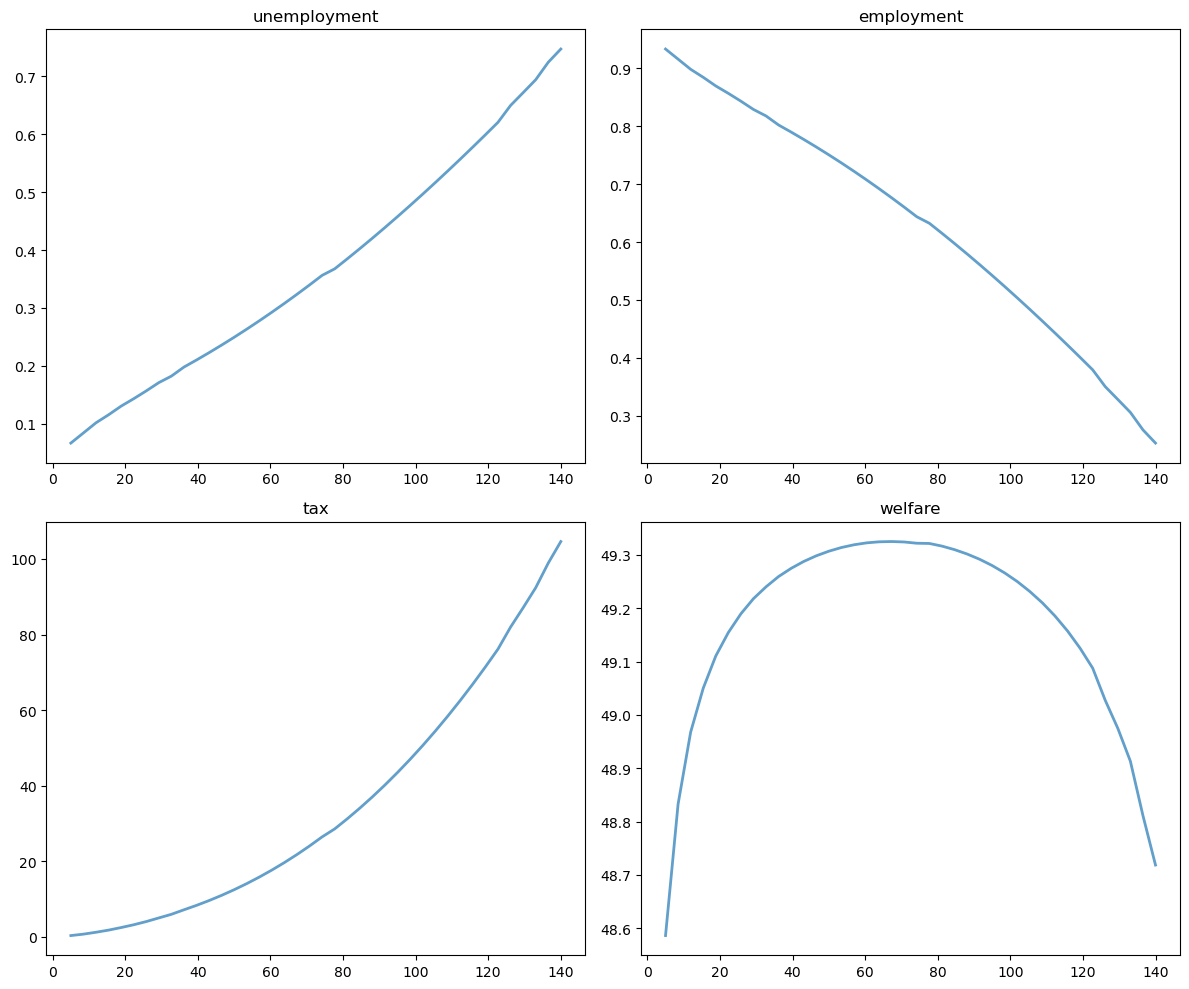
Welfare first increases and then decreases as unemployment benefits rise.
The level that maximizes steady state welfare is approximately 62.
71.4. Exercises#
Exercise 71.1
How does the welfare-maximizing level of unemployment compensation \(c\) change with the job separation rate \(\alpha\)?
Compute and plot the optimal \(c\) (the value that maximizes welfare) for a range of separation rates \(\alpha\) from 0.01 to 0.04.
For each \(\alpha\) value, find the optimal \(c\) by computing welfare across the range of \(c\) values and selecting the maximum.
Solution
Here is one solution:
# Range of separation rates to explore (wider range, fewer points)
α_values = jnp.linspace(0.01, 0.04, 8)

# We'll store the optimal c for each α
optimal_c_values = []

# Use a finer grid for c values to get better resolution
c_vec_fine = jnp.linspace(5, 140, 150)

for α_val in α_values:
    # Create economy parameters with this α
    params_α = create_economy(α=α_val)

    # Create wage distribution
    w_vec_α, p_vec_α = create_wage_distribution(
        params_α.max_wage, params_α.wage_grid_size, params_α.log_wage_mean
    )

    # Compute welfare for each c value
    welfare_values = []
    for c in c_vec_fine:
        t = find_balanced_budget_tax(c, params_α, w_vec_α, p_vec_α)
        e_rate, u_rate, welfare = compute_steady_state_quantities(
            c, t, params_α, w_vec_α, p_vec_α
        )
        welfare_values.append(welfare)

    # The welfare function is very flat near its maximum.
    # Using argmax on a single point can be unstable due to numerical noise.
    # Instead, we find all c values within 99.9% of maximum welfare and
    # compute their weighted average (centroid). This gives a more stable
    # estimate of the optimal unemployment compensation level.
    welfare_array = jnp.array(welfare_values)
    max_welfare = jnp.max(welfare_array)
    threshold = 0.999 * max_welfare
    near_optimal_mask = welfare_array >= threshold

    # Compute weighted average of c values in the near-optimal region
    optimal_c = jnp.sum(c_vec_fine * near_optimal_mask * welfare_array) / \
                jnp.sum(near_optimal_mask * welfare_array)
    optimal_c_values.append(optimal_c)

# Plot the relationship
fig, ax = plt.subplots(figsize=(10, 6))
ax.plot(α_values, optimal_c_values, lw=2, marker='o')
ax.set_xlabel(r'Separation rate $\alpha$')
ax.set_ylabel('Optimal unemployment compensation $c$')
ax.set_title('How optimal unemployment insurance varies with job separation rate')
ax.grid(True, alpha=0.3)
plt.tight_layout()
plt.show()
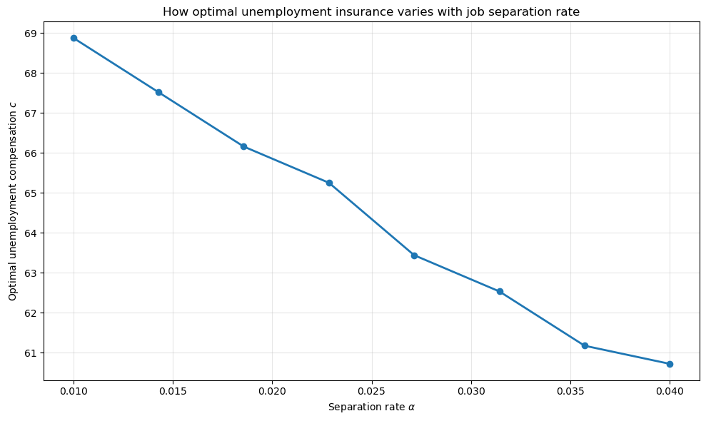
We see that as the separation rate increases (workers lose their jobs more frequently), the welfare-maximizing level of unemployment compensation decreases.
This occurs because higher separation rates increase steady-state unemployment, which raises the tax burden needed to finance unemployment benefits. The optimal policy balances insurance against distortionary taxation.