44. Job Search with Separation and Markov Wages#
This lecture builds on the job search model with separation presented in the previous lecture.
The key difference is that wage offers now follow a Markov chain rather than being independent and identically distributed (IID).
This modification adds persistence to the wage offer process, meaning that today’s wage offer provides information about tomorrow’s offer.
This feature makes the model more realistic, as labor market conditions tend to exhibit serial correlation over time.
In addition to what’s in Anaconda, this lecture will need the following libraries
!pip install quantecon jax
We use the following imports:
from quantecon.markov import tauchen
import jax.numpy as jnp
import jax
from jax import jit, lax
from typing import NamedTuple
import matplotlib.pyplot as plt
from functools import partial
44.1. Model Setup#
Each unemployed agent receives a wage offer \(w\) from a finite set
Wage offers follow a Markov chain with transition matrix \(P\)
Jobs terminate with probability \(\alpha\) each period (separation rate)
Unemployed workers receive compensation \(c\) per period
Future payoffs are discounted by factor \(\beta \in (0,1)\)
44.2. Decision Problem#
When unemployed and receiving wage offer \(w\), the agent chooses between:
Accept offer \(w\): Become employed at wage \(w\)
Reject offer: Remain unemployed, receive \(c\), get new offer next period
44.3. Value Functions#
let \(v_u(w)\) be the value of being unemployed when current wage offer is \(w\)
let \(v_e(w)\) be the value of being employed at wage \(w\)
44.4. Bellman Equations#
The unemployed worker’s value function satisfies the Bellman equation
The employed worker’s value function satisfies the Bellman equation
44.5. Computational Approach#
We use the following approach to solve this problem.
(As usual, for a function \(h\) we set \((Ph)(w) = \sum_{w'} h(w') P(w,w')\).)
Use the employed worker’s Bellman equation to express \(v_e\) in terms of \(Pv_u\):
Substitute into the unemployed agent’s Bellman equation to get:
Use value function iteration to solve for \(v_u\)
Compute optimal policy: accept if \(v_e(w) ≥ c + β(Pv_u)(w)\)
The optimal policy turns out to be a reservation wage strategy: accept all wages above some threshold.
44.6. Code#
First, we implement the successive approximation algorithm.
This algorithm takes an operator \(T\) and an initial condition and iterates until convergence.
We will use it for value function iteration.
@partial(jit, static_argnums=(0,))
def successive_approx(
        T,                         # Operator (callable) - marked as static
        x_0,                       # Initial condition
        tolerance: float = 1e-6,   # Error tolerance
        max_iter: int = 100_000,   # Max iteration bound
    ):
    """Computes the approximate fixed point of T via successive
    approximation using lax.while_loop."""

    def cond_fn(carry):
        x, error, k = carry
        return (error > tolerance) & (k <= max_iter)

    def body_fn(carry):
        x, error, k = carry
        x_new = T(x)
        error = jnp.max(jnp.abs(x_new - x))
        return (x_new, error, k + 1)

    initial_carry = (x_0, tolerance + 1, 1)
    x_final, _, _ = lax.while_loop(cond_fn, body_fn, initial_carry)

    return x_final
Next let’s set up a Model class to store information needed to solve the model.
We include P_cumsum, the row-wise cumulative sum of the transition matrix, to
optimize the simulation – the details are explained below.
class Model(NamedTuple):
    n: int
    w_vals: jnp.ndarray
    P: jnp.ndarray
    P_cumsum: jnp.ndarray  # Cumulative sum of P for efficient sampling
    β: float
    c: float
    α: float
The function below holds default values and creates a Model instance:
def create_js_with_sep_model(
        n: int = 200,          # wage grid size
        ρ: float = 0.9,        # wage persistence
        ν: float = 0.2,        # wage volatility
        β: float = 0.96,       # discount factor
        α: float = 0.05,       # separation rate
        c: float = 1.0         # unemployment compensation
    ) -> Model:
    """
    Creates an instance of the job search model with separation.

    """
    mc = tauchen(n, ρ, ν)
    w_vals, P = jnp.exp(jnp.array(mc.state_values)), jnp.array(mc.P)
    P_cumsum = jnp.cumsum(P, axis=1)
    return Model(n, w_vals, P, P_cumsum, β, c, α)
Here’s the Bellman operator for the unemployed worker’s value function:
@jit
def T(v: jnp.ndarray, model: Model) -> jnp.ndarray:
    """The Bellman operator for the value of being unemployed."""
    n, w_vals, P, P_cumsum, β, c, α = model
    d = 1 / (1 - β * (1 - α))
    accept = d * (w_vals + α * β * P @ v)
    reject = c + β * P @ v
    return jnp.maximum(accept, reject)
The next function computes the optimal policy under the assumption that \(v\) is the value function:
@jit
def get_greedy(v: jnp.ndarray, model: Model) -> jnp.ndarray:
    """Get a v-greedy policy."""
    n, w_vals, P, P_cumsum, β, c, α = model
    d = 1 / (1 - β * (1 - α))
    accept = d * (w_vals + α * β * P @ v)
    reject = c + β * P @ v
    σ = accept >= reject
    return σ
Here’s a routine for value function iteration, as well as a second routine that computes the reservation wage.
The second routine requires a policy function, which we will typically obtain by
applying the vfi function.
def vfi(model: Model):
    """Solve by VFI."""
    v_init = jnp.zeros(model.w_vals.shape)
    v_star = successive_approx(lambda v: T(v, model), v_init)
    σ_star = get_greedy(v_star, model)
    return v_star, σ_star


def get_reservation_wage(σ: jnp.ndarray, model: Model) -> float:
    """
    Calculate the reservation wage from a given policy.

    Parameters:
    - σ: Policy array where σ[i] = True means accept wage w_vals[i]
    - model: Model instance containing wage values

    Returns:
    - Reservation wage (lowest wage for which policy indicates acceptance)
    """
    n, w_vals, P, P_cumsum, β, c, α = model

    # Find all wage indices where policy indicates acceptance
    accept_indices = jnp.where(σ == 1)[0]

    if len(accept_indices) == 0:
        return jnp.inf  # Agent never accepts any wage

    # Return the lowest wage that is accepted
    return w_vals[accept_indices[0]]
44.7. Computing the Solution#
Let’s solve the model:
model = create_js_with_sep_model()
n, w_vals, P, P_cumsum, β, c, α = model
v_star, σ_star = vfi(model)
Next we compute some related quantities, including the reservation wage.
d = 1 / (1 - β * (1 - α))
accept = d * (w_vals + α * β * P @ v_star)
h_star = c + β * P @ v_star
w_star = get_reservation_wage(σ_star, model)
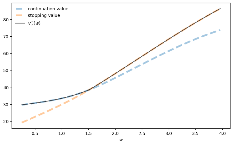
Let’s plot our results.
fig, ax = plt.subplots(figsize=(9, 5.2))
ax.plot(w_vals, h_star, linewidth=4, ls="--", alpha=0.4,
        label="continuation value")
ax.plot(w_vals, accept, linewidth=4, ls="--", alpha=0.4,
        label="stopping value")
ax.plot(w_vals, v_star, "k-", alpha=0.7, label=r"$v_u^*(w)$")
ax.legend(frameon=False)
ax.set_xlabel(r"$w$")
plt.show()
44.8. Sensitivity Analysis#
Let’s examine how reservation wages change with the separation rate.
α_vals: jnp.ndarray = jnp.linspace(0.0, 1.0, 10)

w_star_vec = jnp.empty_like(α_vals)
for (i_α, α) in enumerate(α_vals):
    model = create_js_with_sep_model(α=α)
    v_star, σ_star = vfi(model)
    w_star = get_reservation_wage(σ_star, model)
    w_star_vec = w_star_vec.at[i_α].set(w_star)

fig, ax = plt.subplots(figsize=(9, 5.2))
ax.plot(α_vals, w_star_vec, linewidth=2, alpha=0.6,
        label="reservation wage")
ax.legend(frameon=False)
ax.set_xlabel(r"$\alpha$")
ax.set_ylabel(r"$w$")
plt.show()
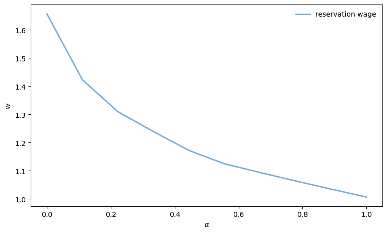
Can you provide an intuitive economic story behind the outcome that you see in this figure?
44.9. Employment Simulation#
Now let’s simulate the employment dynamics of a single agent under the optimal policy.
Note that, when simulating the Markov chain for wage offers, we need to draw from the distribution in each row of \(P\) many times.
To do this, we use the inverse transform method: draw a uniform random variable and find where it falls in the cumulative distribution.
This is implemented via jnp.searchsorted on the precomputed cumulative sum
P_cumsum, which is much faster than recomputing the cumulative sum each time.
The function update_agent advances the agent’s state by one period.
@jit
def update_agent(key, is_employed, wage_idx, model, σ):
    """
    Updates an agent by one period.  Updates their employment status and their
    current wage (stored by index).

    Agents who lose their job that pays wage w receive a new draw in the next
    period via the probabilites in P(w, .)

    """
    n, w_vals, P, P_cumsum, β, c, α = model

    key1, key2 = jax.random.split(key)
    # Use precomputed cumulative sum for efficient sampling
    new_wage_idx = jnp.searchsorted(
        P_cumsum[wage_idx, :], jax.random.uniform(key1)
    )
    separation_occurs = jax.random.uniform(key2) < α
    accepts = σ[wage_idx]

    # If employed: status = 1 if no separation, 0 if separation
    # If unemployed: status = 1 if accepts, 0 if rejects
    final_employment = jnp.where(
        is_employed,
        1 - separation_occurs.astype(jnp.int32),  # employed path
        accepts.astype(jnp.int32)                 # unemployed path
    )

    # If employed: wage = current if no separation, new if separation
    # If unemployed: wage = current if accepts, new if rejects
    final_wage = jnp.where(
        is_employed,
        jnp.where(separation_occurs, new_wage_idx, wage_idx),  # employed path
        jnp.where(accepts, wage_idx, new_wage_idx)             # unemployed path
    )

    return final_employment, final_wage
Here’s a function to simulate the employment path of a single agent.
def simulate_employment_path(
        model: Model,     # Model details
        σ: jnp.ndarray,   # Policy (accept/reject for each wage)
        T: int = 2_000,   # Simulation length
        seed: int = 42    # Set seed for simulation
    ):
    """
    Simulate employment path for T periods starting from unemployment.

    """
    key = jax.random.PRNGKey(seed)
    # Unpack model
    n, w_vals, P, P_cumsum, β, c, α = model

    # Initial conditions
    is_employed = 0
    wage_idx = 0

    wage_path_list = []
    employment_status_list = []

    for t in range(T):
        wage_path_list.append(w_vals[wage_idx])
        employment_status_list.append(is_employed)

        key, subkey = jax.random.split(key)
        is_employed, wage_idx = update_agent(
            subkey, is_employed, wage_idx, model, σ
        )

    return jnp.array(wage_path_list), jnp.array(employment_status_list)
Let’s create a comprehensive plot of the employment simulation:
model = create_js_with_sep_model()

# Calculate reservation wage for plotting
v_star, σ_star = vfi(model)
w_star = get_reservation_wage(σ_star, model)

wage_path, employment_status = simulate_employment_path(model, σ_star)

fig, (ax1, ax2, ax3) = plt.subplots(3, 1, figsize=(8, 6))

# Plot employment status
ax1.plot(employment_status, 'b-', alpha=0.7, linewidth=1)
ax1.fill_between(
    range(len(employment_status)), employment_status, alpha=0.3, color='blue'
)
ax1.set_ylabel('employment status')
ax1.set_title('Employment path (0=unemployed, 1=employed)')
ax1.set_xticks((0, 1))
ax1.set_ylim(-0.1, 1.1)

# Plot wage path with employment status coloring
ax2.plot(wage_path, 'b-', alpha=0.7, linewidth=1)
ax2.axhline(y=w_star, color='black', linestyle='--', alpha=0.8,
           label=f'Reservation wage: {w_star:.2f}')
ax2.set_xlabel('time')
ax2.set_ylabel('wage')
ax2.set_title('Wage path (actual and offers)')
ax2.legend()

# Plot cumulative fraction of time unemployed
unemployed_indicator = (employment_status == 0).astype(int)
cumulative_unemployment = (
    jnp.cumsum(unemployed_indicator) /
    jnp.arange(1, len(employment_status) + 1)
)

ax3.plot(cumulative_unemployment, 'r-', alpha=0.8, linewidth=2)
ax3.axhline(y=jnp.mean(unemployed_indicator), color='black',
            linestyle='--', alpha=0.7,
            label=f'Final rate: {jnp.mean(unemployed_indicator):.3f}')
ax3.set_xlabel('time')
ax3.set_ylabel('cumulative unemployment rate')
ax3.set_title('Cumulative fraction of time spent unemployed')
ax3.legend()
ax3.set_ylim(0, 1)

plt.tight_layout()
plt.show()
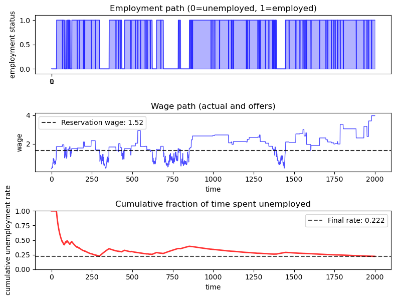
The simulation helps to visualize outcomes associated with this model.
The agent follows a reservation wage strategy.
Often the agent loses her job and immediately takes another job at a different wage.
This is because she uses the wage \(w\) from her last job to draw a new wage offer via \(P(w, \cdot)\), and positive correlation means that a high current \(w\) is often leads a high new draw.
44.10. The Ergodic Property#
Below we examine cross-sectional unemployment.
In particular, we will look at the unemployment rate in a cross-sectional simulation and compare it to the time-average unemployment rate, which is the fraction of time an agent spends unemployed over a long time series.
We will see that these two values are approximately equal – if fact they are exactly equal in the limit.
The reason is that the process \((s_t, w_t)\), where
\(s_t\) is the employment status and
\(w_t\) is the wage
is Markovian, since the next pair depends only on the current pair and iid randomness, and ergodic.
Ergodicity holds as a result of irreducibility.
Indeed, from any (status, wage) pair, an agent can eventually reach any other (status, wage) pair.
This holds because:
Unemployed agents can become employed by accepting offers
Employed agents can become unemployed through separation (probability \(\alpha\))
The wage process can transition between all wage states (because \(P\) is itself irreducible)
These properties ensure the chain is ergodic with a unique stationary distribution \(\pi\) over states \((s, w)\).
For an ergodic Markov chain, the ergodic theorem guarantees that time averages = ensemble averages.
In particular, the fraction of time a single agent spends unemployed (across all wage states) converges to the cross-sectional unemployment rate:
This holds regardless of initial conditions – provided that we burn in the cross-sectional distribution (run it forward in time from a given initial cross section in order to remove the influence of that initial condition).
As a result, we can study steady-state unemployment either by:
Following one agent for a long time (time average), or
Observing many agents at a single point in time (cross-sectional average)
Often the second approach is better for our purposes, since it’s easier to parallelize.
44.11. Cross-Sectional Analysis#
Now let’s simulate many agents simultaneously to examine the cross-sectional unemployment rate.
We first create a vectorized version of update_agent to efficiently update all agents in parallel:
# Create vectorized version of update_agent
update_agents_vmap = jax.vmap(
    update_agent, in_axes=(0, 0, 0, None, None)
)
Next we define the core simulation function, which uses lax.fori_loop to efficiently iterate many agents forward in time:
@partial(jit, static_argnums=(3, 4))
def _simulate_cross_section_compiled(
        key: jnp.ndarray,
        model: Model,
        σ: jnp.ndarray,
        n_agents: int,
        T: int
    ):
    """JIT-compiled core simulation loop using lax.fori_loop.
    Returns only the final employment state to save memory."""
    n, w_vals, P, P_cumsum, β, c, α = model

    # Initialize arrays
    wage_indices = jnp.zeros(n_agents, dtype=jnp.int32)
    is_employed = jnp.zeros(n_agents, dtype=jnp.int32)

    def update(t, loop_state):
        key, is_employed, wage_indices = loop_state

        # Shift loop state forwards - more efficient key generation
        key, subkey = jax.random.split(key)
        agent_keys = jax.random.split(subkey, n_agents)

        is_employed, wage_indices = update_agents_vmap(
            agent_keys, is_employed, wage_indices, model, σ
        )

        return key, is_employed, wage_indices

    # Run simulation using fori_loop
    initial_loop_state = (key, is_employed, wage_indices)
    final_loop_state = lax.fori_loop(0, T, update, initial_loop_state)

    # Return only final employment state
    _, final_is_employed, _ = final_loop_state
    return final_is_employed


def simulate_cross_section(
        model: Model,
        n_agents: int = 100_000,
        T: int = 200,
        seed: int = 42
    ) -> float:
    """
    Simulate employment paths for many agents and return final unemployment rate.

    Parameters:
    - model: Model instance with parameters
    - n_agents: Number of agents to simulate
    - T: Number of periods to simulate
    - seed: Random seed for reproducibility

    Returns:
    - unemployment_rate: Fraction of agents unemployed at time T
    """
    key = jax.random.PRNGKey(seed)

    # Solve for optimal policy
    v_star, σ_star = vfi(model)

    # Run JIT-compiled simulation
    final_employment = _simulate_cross_section_compiled(
        key, model, σ_star, n_agents, T
    )

    # Calculate unemployment rate at final period
    unemployment_rate = 1 - jnp.mean(final_employment)

    return unemployment_rate
This function generates a histogram showing the distribution of employment status across many agents:
def plot_cross_sectional_unemployment(model: Model, t_snapshot: int = 200,
                                     n_agents: int = 20_000):
    """
    Generate histogram of cross-sectional unemployment at a specific time.

    Parameters:
    - model: Model instance with parameters
    - t_snapshot: Time period at which to take the cross-sectional snapshot
    - n_agents: Number of agents to simulate
    """
    # Get final employment state directly
    key = jax.random.PRNGKey(42)
    v_star, σ_star = vfi(model)
    final_employment = _simulate_cross_section_compiled(
        key, model, σ_star, n_agents, t_snapshot
    )

    # Calculate unemployment rate
    unemployment_rate = 1 - jnp.mean(final_employment)

    fig, ax = plt.subplots(figsize=(8, 5))

    # Plot histogram as density (bars sum to 1)
    weights = jnp.ones_like(final_employment) / len(final_employment)
    ax.hist(final_employment, bins=[-0.5, 0.5, 1.5],
            alpha=0.7, color='blue', edgecolor='black',
            density=True, weights=weights)

    ax.set_xlabel('employment status (0=unemployed, 1=employed)')
    ax.set_ylabel('density')
    ax.set_title(f'Cross-sectional distribution at t={t_snapshot}, ' +
                 f'unemployment rate = {unemployment_rate:.3f}')
    ax.set_xticks([0, 1])

    plt.tight_layout()
    plt.show()
Now let’s compare the time-average unemployment rate (from a single agent’s long simulation) with the cross-sectional unemployment rate (from many agents at a single point in time):
model = create_js_with_sep_model()
cross_sectional_unemp = simulate_cross_section(
    model, n_agents=20_000, T=200
)

time_avg_unemp = jnp.mean(unemployed_indicator)
print(f"Time-average unemployment rate (single agent): "
      f"{time_avg_unemp:.4f}")
print(f"Cross-sectional unemployment rate (at t=200): "
      f"{cross_sectional_unemp:.4f}")
print(f"Difference: {abs(time_avg_unemp - cross_sectional_unemp):.4f}")
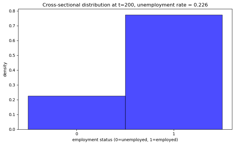
Time-average unemployment rate (single agent): 0.2215
Cross-sectional unemployment rate (at t=200): 0.2257
Difference: 0.0042
Now let’s visualize the cross-sectional distribution:
plot_cross_sectional_unemployment(model)
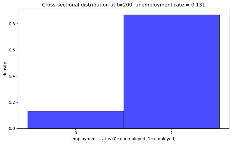
44.12. Cross-Sectional Analysis with Lower Unemployment Compensation (c=0.5)#
Let’s examine how the cross-sectional unemployment rate changes with lower unemployment compensation:
model_low_c = create_js_with_sep_model(c=0.5)
plot_cross_sectional_unemployment(model_low_c)
44.13. Exercises#
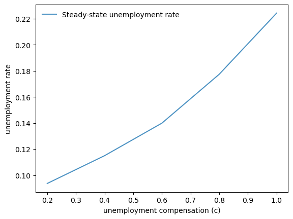
Exercise 44.1
Create a plot that shows how the steady state cross-sectional unemployment rate changes with unemployment compensation.
Solution
We compute the steady-state unemployment rate for different values of unemployment compensation:
c_values = 1.0, 0.8, 0.6, 0.4, 0.2
rates = []
for c in c_values:
    model = create_js_with_sep_model(c=c)
    unemployment_rate = simulate_cross_section(model)
    rates.append(unemployment_rate)

fig, ax = plt.subplots()
ax.plot(
    c_values, rates, alpha=0.8,
    linewidth=1.5, label='Steady-state unemployment rate'
)
ax.set_xlabel('unemployment compensation (c)')
ax.set_ylabel('unemployment rate')
ax.legend(frameon=False)
plt.show()